Introduction
Quick start
The best way to get started quickly is to load any of the example projects in the Examples sub-folder of your TurbulenceFD installation and experiment with the settings. To create a scene from scratch, follow the following steps:
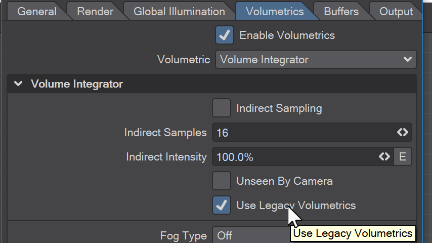
- Press Ctrl+P to open Render Properties or go the the Render Properties button on the Render tab. In there, go to the Volumetrics tab and check Use Legacy Volumetrics
- Select Add Container from the TurbulenceFD menu
- To define the shape of your emitter
- load an .lwo object
- or create geometry using Modeler, Layout's Modeler Tools/Geometry or the new Procedural Geometry tools
- or create a particle system using Items/Dynamic Obj/Particle
- With the new object selected, choose Make Emitter from the TurbulenceFD menu
- In the Channels tab of the Fluid Emitter popup, set Temperature to 1.0
- Press the Start button in the TurbulenceFD main dialog
- A dialog with a progress bar appears as the simulation is being computed.
- After simulating, you can render the result
Painting Fluid
One important aspect of controlling a fluid simulation (if not the most important one) is to create the right emitter setup.
You can think of the emitter as a brush used to paint a pixel image. In fact, the container works pretty much like a 3D pixel image. You paint into one or more of the fluid channels (similar to painting into the RGB and/or A channels of an image) using emitters.
The fluid simulation will then add velocities that let your "paint" flow, curl and/or expand. Essentially the result will be what you painted at the source. You'll want to try various settings for the emitter texture scale, octaves and contrast. Maybe use several small objects instead of a single big one, use particles, animate the intensity of the emission, etc.
You can start by using only the temperature channel (disable the others) and see what different effects you can get just by varying the emission pattern and animation. You may not even need more than one channel for an effect - even in a high-quality production.
Fire simulation
Fire can be simulated in several ways. All you need is one or two fields as a basis to set up your fire shader, which is what you will most likely spend the most time with. You can even use the most straightforward density simulation and turn it into a nice flame by only using good shading parameters. The density-based flame example project shows how this works. See the next section for more details on shading fire.
There are several ways to get more control over your fire simulation. They are based on the Fuel channel. Objects can emit fuel that will burn if the temperature at a voxel is above the Ignition Temperature. When fuel burns, the air heats up and expands, as specified by the Expansion parameter. This is the essential control for explosions and large fireballs. Another effect of burning fuel is the Heat Creation and Density Creation. These parameters control how much is added to the temperature and density channels per unit of burnt fuel. Heat Creation is how a fire keeps itself burning, that is keeps the temperature above the ignition temperature after the initial ignition.
Fuel may move slower than the rest of the fluid. This gives you some additional control over the shape of the flames. So does the Fuel Diffusion parameter, which will essentially blur the fuel field, letting fuel spread slowly in all directions regardless of the movement in the fluid.
The Fire channel provides an alternative channel to render fire. Fire values are large wherever fuel burns and diminish the farther away from the burning fuel they are. This creates a field that allows you to shade the flame based on the distance to the flame core. The next section will go into more detail on shading fire.
Shading fire
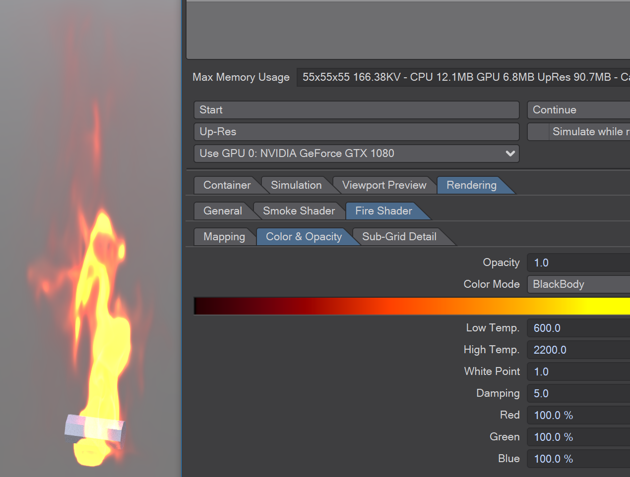
From a visual perspective, fire is essentially hot gas and soot particles that emit light. Most flames consist mostly of soot which is Carbon. Carbon is what is called a Black Body. A Black Body absorbs all light that hits it, hence it is black. However, when its temperature rises to over about 600 Kelvin, it starts to emit light in a very characteristic way. This is where the familiar red/orange/yellow/white colors come from. Because fire mostly consists of soot particles, this is what dominates the color of flames.
Since soot particles emit the light of a flame, that means that the more soot particles there are, the brighter the flame will be. On the other hand, since Black Bodies also absorb light, more soot particles also make the flame more opaque. These two effects are exactly what is controlled by the Opacity group of the Fire Shader. This is what you use to control the shape of the flame.
To control the color you have two options. One is to specify a color gradient directly and the other is to use the physical model that describes the colors of a radiating Black Body. The latter will give you an easy way to obtain realistic colors, while the former gives you full artistic freedom. When using the custom gradient, take care that you use a high dynamic range of colors (also make sure that the Clamp checkbox is not checked). Look at the intensity values of the default color gradient as an example. It actually has a constant orange color. Only the intensity runs from 0% to 2000%.
As mentioned above, you can shade fire using several different simulation channels. The density-based flame example uses the temperature field to drive the color and the density channel for the opacity. While the fuel-based flame shows pretty much the same using the Fuel and Fire channels. The Fuel channel gives you more freedom to simulate a reaction, but it behaves the same when it comes to shading. In these examples, the mapping of the Opacity group creates the typical flame shape. A rising plume of fuel will only burn at the outer contour where there is enough oxygen. That means that most light is also emitted only from these areas. The mapping function curve exploits the property of Density and Fire fields with large values inside the plume/flame and smaller values outside. By creating a peak in the mapping you specify where the surface of the flame should be that emits most of the light. See the F-Curve editor for more details on how you can design mapping curves.
You can also use the Fire channel to drive the color, the opacity or both. You can even shade flames without using an opacity channel at all - note that in this case, you won't have alpha information to composite your flame later on. You can still composite such a flame by using the brightness of the flame as a matte channel - remember that the brighter the flame is, the more soot particles there are and the more opaque the flame will be.
Fluid Emitter tabs
Container tabs
Menus
There are several menus, and panels inside of menus, in TurbulenceFD. It is important to understand not only what they do but their relationships to each other. Below is a breakdown of each menu type and its basic purpose. Each menu button will bring up their respective menu panels. Let's go through these below.
Containers
Opens the container control window that holds the list of fluid containers, the Container Parameters and the simulation controls.
Container Parameters
Max Memory Usage:
This field shows the maximum resolution (in voxels) that the container can use as well as the amounts of memory that it would use in this case. How much the simulation will actually need depends on how the simulation grows over time.
Here is an example:
386x649x395 99.0MV - CPU 7.9GB GPU 3.7GB UpRes 62.4GB - Cache/F: 1.9GB UpRes 14.9GB
The first section shows the maximum dimensions of the container in voxels and the total number of MegaVoxels or Million Voxels (MV).
The middle section shows the amount of memory the simulation will at most require when run on the CPU, the GPU or in Up-Res mode.
The last section shows the maximum size a single cache frame would have on disk without compression for a normal simulation and an Up-Res pass.
When starting the simulation, TurbulenceFD will warn you if the available memory would not suffice would the simulation take up the whole container. You can ignore the warning if you know that your simulation will stay small enough or if you're keeping an eye on the simulation progress, so you can abort the simulation if necessary. When running simulations un-supervised, it's a good idea to make sure the container dimensions and simulation settings are chosen such that the available memory is sufficient.
If the available memory is exceeded, the machine will most likely become unresponsive and you may have to reboot your system.
- Start - Simulate the fluids in this container from the beginning of the selected frame range (see Simulation/Timing/Frame Range).
- Continue - Continues a simulation after the last simulation state. This last state is always saved when the simulation stops - either because you clicked the Stop button or because all frames from the selected range have been simulated. This also allows you to add more frames at the end of the range.
- Up-Res - Post-processes a simulation to increase the resolution and add more detail. A new cache directory will be created using the name of the current cache with the word "upres" appended. You can switch back to the previous cache using the Container/Cache Directory button.
See the Simulation/Up-Res tab for more options.
This post-process is faster than simulating at a high resolution in the first place. It will also retain the shape of the lores simulation and only add small details that couldn't be resolved on the lores grid before. - Simulate while rendering scene - If checked, the simulation will be run as needed while rendering the scene. This is somewhat faster than simulating and rendering in two passes since the caches don't have to be loaded from disk. With lores camera settings, this is also useful as a previewing mechanism while working on the simulation.
- Use CPUs/GPU - If you have supported GPUs, this drop-down list will let you select which one to use. See GPU Simulation for more details about fluid simulation on GPUs.
If "Use CPUs" is selected, all available CPU cores will be used instead.
F-Curve - Fluid Curve Editor
One of the most important aspects of volume shading is the choice of a transfer function.
This function assigns a color and opacity to every input value. It is the shader's job to define such a transfer function. In order to do this, both shaders use a form of intensity mapping. While the way color is determined differs for smoke and fire, in both shaders the intensity mapping is basically the black-and-white version of the transfer function.
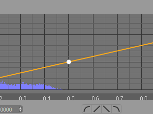
Linear
TurbulenceFD features a special purpose function curve (f-curve) editor that allows for convenient and accurate control of the transfer function by the artist. Working with this editor is very similar to post-processing images with color correction. If you have any experience in that area, this will be familiar to you.
A linear mapping, as shown in the image above, makes color and opacity scale proportional to the input values. In many cases we want to cut off some parts or amplify others, though.
For example, for smoke shading we might want to have a smaller range of thickness (or opacity) that the smoke can take on. That is, the thickness should not fall off linearly with the density, but sustain a high value and then fall off quickly and the low end of the density range as shown in the image below.
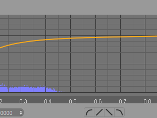
Biased
To assist with the design of the mapping function, the editor shows a histogram of the input values as a backdrop. For example, in the image above we can see that there are no input values above 0.5, so we should focus our mapping function on the values that are actually in the container. Of course, the value distribution will change from frame to frame depending on your simulation, so you will have to look at the histogram as it changes over time and design a mapping function accordingly.
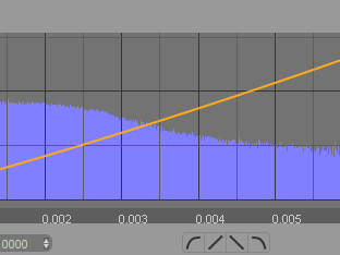
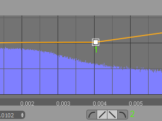
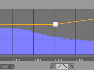
Zoomed
It is often necessary to create very subtle changes to the mapping function to obtain a certain look. Note the value ranges on the X and Y axes in the image above. The editor has been zoomed in to show the fine details at the low end of the input value range. The histogram shows us that there are still significant changes at this scale and by increasing the intensity for this range (about 0.001 to 0.004) we will get a big visual difference.
Fire shading
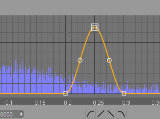
For fire shading, we usually want only a narrow band around the surface of the flame to be visible and luminous. We can do this by defining a small peak in the fire shader's opacity mapping as shown in the image below.
Fine-tuning
With different f-curve designs, we can achieve a wide range of looks. Make smoke contours sharper by suppressing low-density values, fill the inside of a flame by extending the above peak to the right, etc.
Selecting and manipulating
The following image shows the various controls of the editor:
- select and drag knots (1) using the LMB
- add new knots using the RMB
- select multiple knots by holding down shift while left-clicking and dragging the mouse to span a selection rectangle
- move selected knots (1) by left-clicking on any of them and dragging them to their new position
- define smooth or linear tangents for the knots using the tangent buttons (2)
- delete selected knots by pressing the delete button on the toolbar (3) or the delete key
- bend a curve segment (change the bias) by left-clicking a segment handle (4) and moving the mouse horizontally
- change all these values using the value input boxes (5)
- adjust the scale of the histogram using the blue slider on the right (6)
- toggle the histogram on and off using the histogram button (7)
- use the mouse wheel or zoom button (8) to zoom horizontally or vertically when holding Shift at the same time
- use the MMB or the translate button (9) to translate the view
GPU simulation
Fluid Simulation needs quite a bit of processing power. Mostly because there is a huge amount of data to be pushed around. This makes memory bandwidth the most important factor for simulation speed. Today's fastest memory interfaces are found in GPUs - about 10 times faster than those of CPUs. Coupled with the appropriate amount of parallel computing power, GPUs are the ideal type of processor for fluid simulation.
TurbulenceFD makes use of GPUs for its simulation pipeline. Unlike some GPU-accelerated tools, this is not just a stripped-down version of the CPU pipeline. All features are supported at the same quality. In fact, you can switch between CPU and GPU simulation on the fly (see Simulation Window). This is also what TurbulenceFD will do automatically, should it run out of GPU memory. It will then continue the simulation on the CPU.
Supported GPUs
At this time, TurbulenceFD only supports Nvidia GPUs with Compute Capability 2.0 or newer, listed at http://developer.nvidia.com/cuda-gpus
While TurbulenceFD technically works with less than 1GB of GPU memory, a GPU with 4GB or more memory is highly recommended.
Please make sure to use the latest driver for your graphics card and if possible, make use of the Studio edition drivers as they are typically much more stable than Game edition releases.
For the purposes of this documentation and our demonstration content, assume that you will need at least a nVidia GTX 1070 or above graphics card with 8GB (minimum) of VRAM in most cases, in order to simulate them without running into a limited VRAM situation.
Hardware Setup Tips
- At this time, TurbulenceFD can only make use of one GPU per simulation container in a scene. While it is possible to have different GPUs assigned to different containers, only one container can be simulated at a time.
- When choosing a GPU, prefer the one with the most per-GPU memory (note that per-GPU memory for Dual-GPU boards is usually half of the advertised amount)
- Even prefer a slower GPU if it has more memory than an alternative faster GPU (see this post for the rationale behind this advice)
- Ideally use two GPUs: one (possibly smaller one) as primary display GPU and one as a secondary GPU for simulation only.
- When your system has only one GPU and you run large simulations, disable the viewport preview to speed up the simulation.
- If you have a supported GPU but don't have anything to select but "Use CPUs", update your graphics display driver (see Supported GPUs above).
- The larger the voxel size resolution the better the speedup (GPU vs. CPU) will be.
Tweaking Performance
General tips:
- Store/Load the sim caches to/from the fastest drive you have (e.g. an SSD, M.2). Avoid network drives unless you're on a high-end network and file server (10GbE, etc.).
- Make sure your virus scanner does not scan .bcf files on read/write.
- Close all other applications during sim/render.
Simulation Performance:
- Don't run simulations that exceed your available memory.
- Make sure you don't sim and/or cache channels you don't need for rendering.
- Use only low values like 1 or 2 for sub-frame or pressure iteration steps unless you see artifacts.
- Don't use collision objects unless they're essential to your effect.
- Don't use very high-poly objects as emitters. Use low-poly proxies instead.
- Don't use large numbers of octaves for noise on emitters, turbulence, etc. unless you're sure you need them.
- Disable the preview(s) and/or timeline update during simulation.
- When using several emitter objects, parenting them under a null with one emitter tag is faster than adding a separate tag to each object.
To optimize render times, consider this:
- Use Sub-Grid Detail only if absolutely necessary. Use a low or no distance between the Largest and Smallest Scale.
- Avoid sections of mapping curves that have values close to zero. This often happens when strongly bending a curve segment, such that one part of it seems to touch zero, but it actually doesn't.
- Use Voxelized Fast Illumination.
- Lower the Illumination Resolution until you see artifacts.
- For multiple scattering illumination, lower the Depth and Directional Resolution until you see artifacts.
- Make sure Adaptive Step Size is enabled.
- Increase the Step Size and Shadow Step Size until you see artifacts.
- For Motion Blur use a low number of Sub-Steps.
A quick guide to workflow with TurbulenceFD
LightWave Layout is well known for allowing an artist to take many different routes to reach an end result. TurbulenceFD, because of how its various components work together, allows for a very flexible workflow. Generally, there is a basic "start to finish" path which we will discuss here, but there are things that should taken into consideration prior to starting a scene that will make use of TurbulenceFD.
Basic Workflow Concepts - before you start!
Animation of objects in your scene should in most cases be undertaken first, but when TFD is going to be used, your shot or scene design needs to be considerate of a few initial factors.
One of the first considerations is how much an object, ie an emitter/collider or a ParticleFX emitter, moves and how far, over the course of your animation in terms of XYZ space. The reason for this comes down to the minimum TFD Fluid Container size required, the voxel resolution needed for a Fluid Container to encapsulate the fluid being emitted by your emitters, and any wind or pressure considerations that push your fluid around the container all while not clipping the boundaries of the container itself. Furthermore, one must also take into account how many fluid channels will be needed to calculate accurately the effect you want to simulate, within the CPU/GPU and disk space limitations that you have based on your computer system.
Another consideration is how you want your object to emit a fluid. More precisely speaking, through the use of masks applied to an object so that fluid channels emit from a specific portion of the object rather than all of its geometry. If for example, you want to have the tip of a torch or a portion of a floor or wall burning or smoking or a combination of the two, you will need to prepare your object for this either by creating a separate geometry layer that will just emit fluid, or by creating a UV texture that has a white (or greyscale) image applied to it for the area of the object that will emit fluid. We cover this process in our examples so please make sure to check those out.
Finally, object preparation is an important consideration when working with TFD for the purposes of optimization. Lower polygon count objects and objects that are "frozen" or tripled, rather than quads with sub patches - will perform better when it comes to simulation speed. The reason for this is that TurbulenceFD works to create simulations based on the OpenGL polygon evaluation of an object surface or ParticleFX particle emitted, plus a "radius" or distance from the polygon surface or particle point as set in the Emitter Panel. Essentially, low-resolution proxy objects are going to work better for simulation speed than high-poly objects. LightWave Modeler provides tools for doing polygon reduction and there are excellent third-party tools such as Mootool's Polygon Cruncher that work directly with Modeler or in stand-alone mode that can make quick work of doing polygon reduction while retaining a highly-accurate degree of the shape of an object. This is important for things like surface collisions of fluid or emission of fluid along the surface of the proxy object, closely matching a higher resolution version that would be used in your rendering.
Now that these considerations are in mind, let's walk through a quick set up of a scene that makes use of TurbulenceFD. We won't be getting too fancy here, just something simple.
Starting with a Fresh Scene
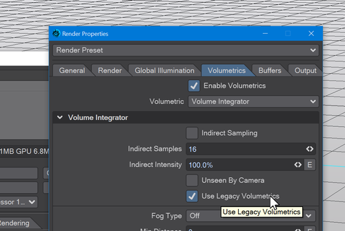
Starting with a fresh scene working in LightWave Layout, we will want to hit ctrl+p to bring up the Render Properties Panel. In the tab labelled "Volumetrics", look for a button in the volume integrator settings, called "Use Legacy Volumetrics" and enable it. For now, TurbulenceFD is classified as a Legacy Volumetric Effect and we need to use this setting for TurbulenceFD to visibly render in VPR, F9, F10 or network renders.
Now that we have this enabled, we can move on to creating our scene.
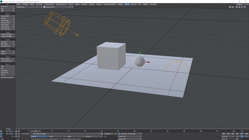
We need some objects to be emitters, collision objects or ParticleFX emitters so let's add something. In the example below, we have created a 5m x 5m ground plane, a 1m cube, resting on the ground and a 250 mm-sized sphere. You can use actual geometry for this or the 2023 Procedural Geometry. You can't use Primitive shapes as emitters or collision objects.
Next, let's animate the box and the sphere over the course of 200 frames. Move your objects around, thinking of where you want your simulation to eventually be.
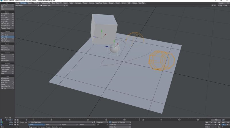
Now that we have some animation on these two objects, let's set them up as TFD Emitters.
There are two ways to tag the objects as TFD emitters. The easiest way is - with one of the objects selected - go to the TurbulenceFD tab at the top of your interface in Layout and look for the button that says TFD Make Emitter. We will do this with the sphere. The other way is to hit the properties button (p) with the object selected, go to the "Appearance" Tab and from the Add Custom Object Dropdown, select Fluid Emitter. For now, though, we will just use the button on the TFD Menu list. Doing so should bring up the Fluid Emitters window with the object listed in the section under Object Name. In our example, that is New Sphere Object. In the displayed General Tab, the defaults are pretty good here but we may want to enable Collision Object, depending on what your animation is doing. So we will do that here as well.
Next, let's select the Cube object and choose the button, Make Collision from the TFD Menu panel in Layout. This will add the cube to the list of objects in the Fluid Emitters window and you will notice that it is already set with the "Collision Object" button enabled. Now let's do the same with the ground plane. At the end of this step, you should see something similar in your list.
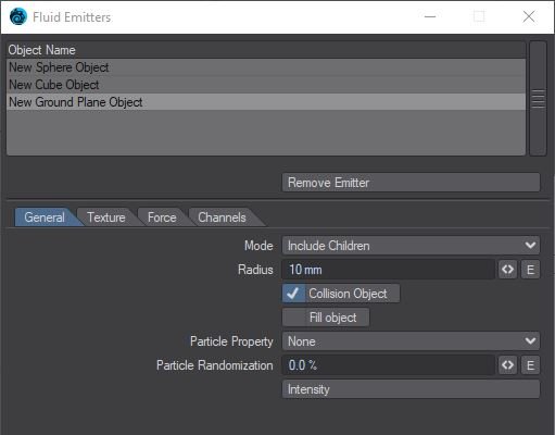
For this next step, we can pretty much leave the ground plane and cube objects alone as they are set as desired in this example. Our interest now is the sphere. Let's select that item in the Object Name list and then move through the panels as we set it up to emit fluid.
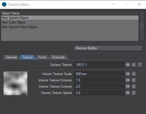
In the Texture Tab, we have five settings, broken up into two areas. The first is called "Surface Texture" with a default of 100% and you will notice it has a value mini-slider to the right of it and an E for envelope, and T for texturing. Should you wish to make use of these functions and want to learn more, we have some example scenes that work with these properties for you to check out. For now, though, the settings we are interested in are in the second section. Let's change Volume Texture Scale to a higher value such as .5m (500mm). You will notice that the white preview of the texture has now become partially covered with gray or darker areas, similar to how the Turbulence texture looks, part of the reason why this tool is called TurbulenceFD. This pattern is what will be "wrapped" around your object as a Fluid emission surface area. The brighter areas will emit fluid at 100% of the value setting in the channels tab, with darker areas going down to black at 0%. If you want to see what this pattern actually does over time, you can scrub through your timeline with the Fluid Emitter window open and the preview box area will change.
Next, we want to set Volume Texture Octaves, Contrast and Speed to different values. You can play around with all of these settings and see what they do to the preview box area and get an idea of how that will affect the emission of Fluid from your object.
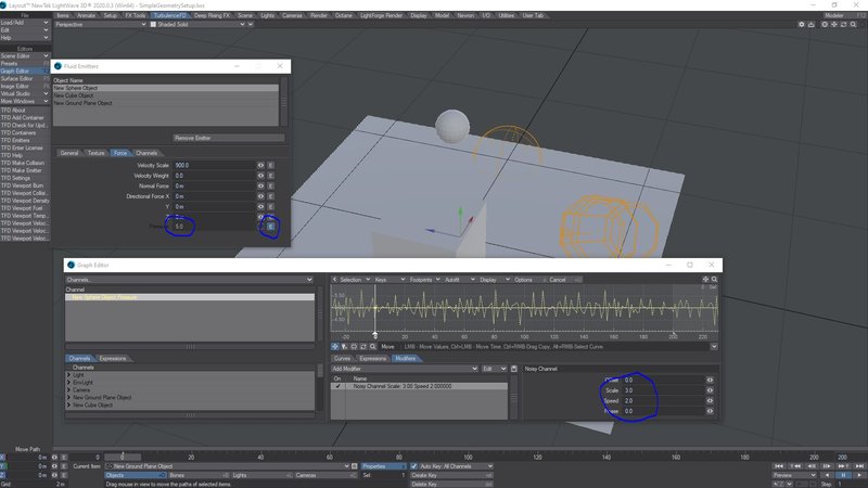
Next up is the "Force" Tab. Look for a setting called "Pressure" and let's change that from the default of 0.0 to something much higher. We can even put an envelope on it if we want and make use of a channel modifier like "Noisy Channel". Here is an example below.
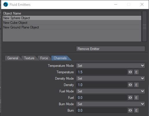
Next, we need to emit some fluid. For that, we will go to the Channels tab. To keep things simple for this example, we will set "Temperature" to 1.5 and "Density" to 1.0. Leave all other settings as their defaults.
Once you have these settings entered, we can move the Fluid Emitters window off to the side or even close it. We can come back to it later if need be. It's time to set up our Fluid Container!
As with Fluid Emitter tags being applied to an object, there are two ways to create a Fluid Container. Fluid Containers in general are really just null objects with the Custom Object Fluid Container tag placed on them in the properties panel for the null object, under the Appearance Tab. Let's take the short route to make a container and simply hit the "TFD Add Container" button in the TurbulenceFD menu. When you hit this button, a "Build Fluid Container" window will pop up with a Title text entry field pre-filled for you with "Fluid Container". You can change this name to whatever you want and then hit the "Ok" button.
Once you do that, you should be presented with something similar to the image below, but we will need to change the settings and placement of the container.
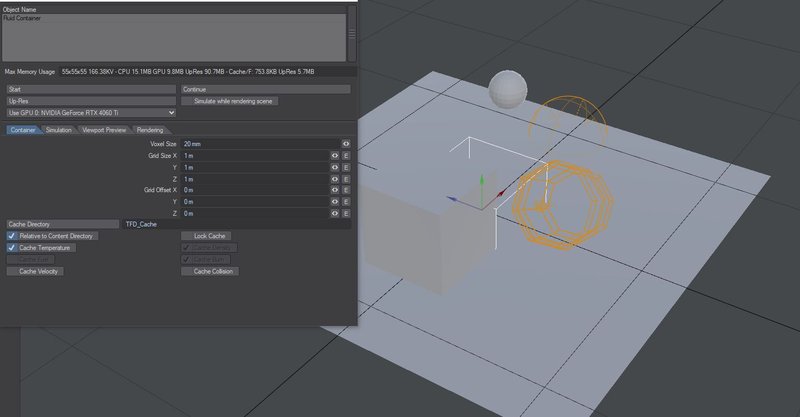
As you can see, the default creation Fluid Container settings have placed the white wire frame "cube" directly in the center of the scene and it is too small to encapsulate our objects. We need to fix this as well as change some other settings immediately. Since we know our ground plane object is 5m x 5m, let's increase the "Grid Size" in this panel to match X and Z, and we will obviously need some height so let's set each value to 5m. This will give us a 5m x 5m x 5m "Fluid Container". We will also need to provide a Grid Off Set value in the Y axis. To get the container to essentially rest on the ground plane, let's use Y=2.5m. We may also want to change the voxel size to 10mm to closely match that of our emitter and collision objects. However, you will notice that the container voxel Max Memory Useage numbers have changed wildly from 1.4GB to 10GB for CPU and from 886.1MB to 6.8GB on the GPU. This is also for only with "Cache Temperature" enabled. We need at least Temperature and Density so these may not be settings that work for you on your system. Alternatively, we can reduce the Max Memory Usage, by increasing the Voxel Size to 15mm. This cuts memory requirements down a lot and because our objects are animated, their chances of "activating" a voxel accurately are pretty good at these settings. Next let's set a location for our Cache Directory, and then move to the simulation tab and make sure we have "Active" enabled on the Density tab. Once you have that set, return to the "Container Tab" and you should see something like this.
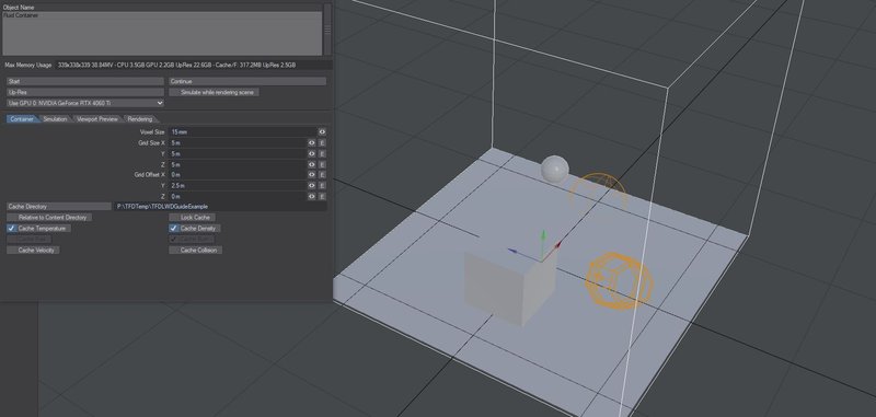
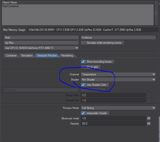
As you can see in the image above, our Fluid Container is now resting on ground, encapsulating the objects in our scene. Next we need to go to the "Viewport Preview" tab and depending on what channel you wish to have visualized in OpenGL (for now TurbulenceFD can only display on type of Fluid Channel in Layout at a time), you will need to select it and a shader for it. For Temperature, select the Shader "Fire Shader" in the drop-down menu. You should have it set to what is shown in the image below.
Now we get to the fun part - Simulation! We can hit the start button here and watch the simulation calculate over the course of our animation. Just make sure to set your Layout Viewport mode to "Textured Shaded Solid" first. If its already set that way, hit "Start". If you are prompted with a "Overwrite Cache?" warning and this is your first time simulating your scene, you can safely ignore this by hitting "Yes".
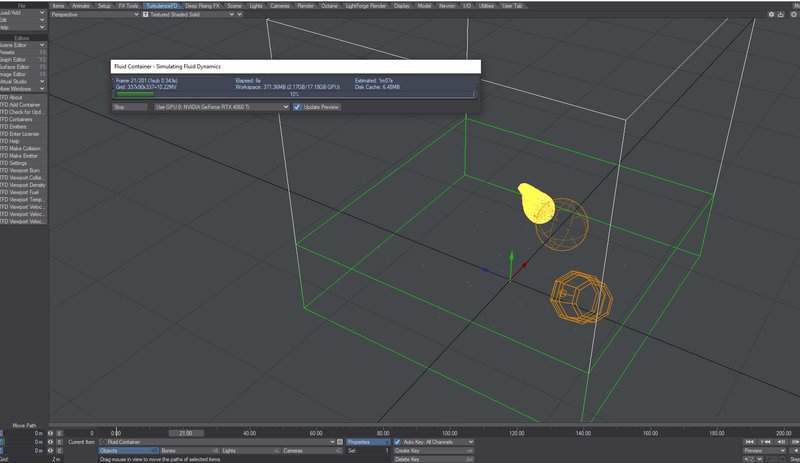
As you can see in the image above, the simulation is calculating and we can see the Fire Shader, applied to the Temperature Channel, emitting from the Sphere. It should, depending on your animation, also interact with the Cube object as it will collide with any channels of fluid emitted by the Sphere. It may be hard to see what it's doing "gas" wise, so if you go back into the Viewport Preview Tab, you can change the Channel and Shader type. Don't be alarmed if some of your objects disappear visually when the simulation is running. They will return once the simulation is complete. TurbulenceFD does this to optimize simulation speed while displaying the update to Layout over time. In some circumstances, such as extremely heavy scenes with lots of items, you may find that you will have to set the appearance back from bounding box or vertex display modes to Texture Shaded Solid in the scene editor manually after a simulation is complete. This is a "quirk" of TurbulenceFD that we hope to resolve in the near future.
Now that we have a simulation, we can move on to shading our temperature and density channels with the Fire and Smoke Shaders respectively so that they show up in render.
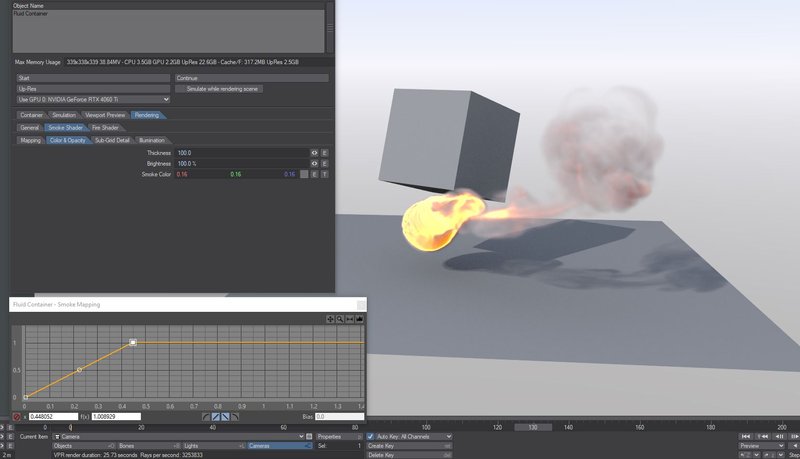
For this next step, let's go to the Rendering Tab in the Fluid Container window and jump to the Smoke Shader sub-tab. The default as you will see is set to "none" in the Channel dropdown menu. Let's change this to Density.
Next, let's change the mapping curve for the density so that the F-Curve end point is brought in on the F-Curve Graph to a little past 0.4 on the X axis and peaking at 1.0 on the Y axis.
After we set that, let's jump to the Color & Opacity sub-tab and set our Thickness to 100.0, leave brightness at its default of 100% but set the smoke color to something much darker such as RGB = 0.16, 0.16, 0.16. We can also remove the Texture (shift-click LMB on the button) to the right of this field as we will not be making use of it and currently there is an issue with this Fluid Channel Gradient that is applied by default, so we can get rid of it entirely.
Turn on VPR and you should see something like this.
We are not done here just yet. We need to set some things in the Sub-Grid Detal sub-panel for our smoke so let's do that now.
In the Sub-Grid Detail Panel, let's increase the Smoke Noise Intensity a little bit to 100 mm from its default of 0 m. Next, let's make sure that our Smoke Noise Smallest Size is set to or below our voxel size. This will ensure that during render over time there is no "popping" in the smoke. This will however increase render times. To help compensate for that, let's move over to the Illumination Tab.
The defaults here are "Voxelized Fast" Scattering, Anisotropy 0.0 and Illumination Resolution set to 100%. We can drop the Illumination Resolution to 75% and you will see that render times decrease significantly. If you are wondering why you are not seeing much smoke, the main reason for this is we didn't really emit a large amount of it in the first place in the Density Channel of our Emitter. We can go back and change this and re-simulate our scene. We are going to do this and set the emitter to push out a higher amount of units of Density rather than 1.5. We will also change the dissipation percentage. So let's do that now and re-simulate the scene and see what we get.
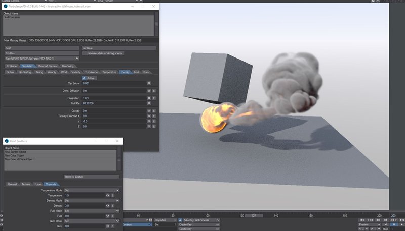
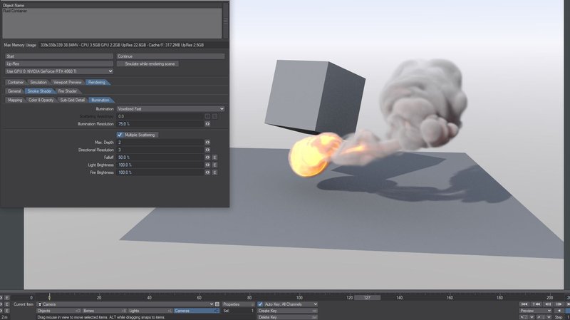
Now we have much more "Smoke" that lives longer as it emits from the Sphere. We can now also start to see the Sub-Grid Detail come out that we set in the Smoke Shader. You will notice however that even with the default Distant and Environment Light in the scene, that the dark areas of the smoke are really dark. To help "illuminate" this problem, we can enable Multiple Scattering and use a few different settings that the defaults. Let's set max depth to 2 and fall off to 50% in the... . It may be wise to turn VPR off for this until you are done, as enabling Multiple Scattering will cause a refresh and lighting calculation based on the settings found in the Multiple Scattering section. Once you are ready with your new settings, you can re-enable VPR. When you do this, a dialog box will appear that shows the multiple scattering calculation taking place. The end result will show your scene with a much more appealing and realistic scattering of light into and through the smoke shader, refracting as it goes, turning those really dark (i.e. black) areas, more naturally gray.
You can definitely see the difference in the image above. Let's move on to the Fire Shader settings in the Fire Shader Sub-tab and then the Sub-Grid Detail tab. Let's increase the Fire Noise Intensity to a value higher than the default of 0m and change up the Fire Noise Smallest Size and Largest Scale values. In order to speed things up for interactivity, we can disable the Smoke Shader and just work on tweaking our Fire Shader values. This will vastly improve your workflow. We will also make some adjustments to the Fire Shader F-Curve while we are at it.
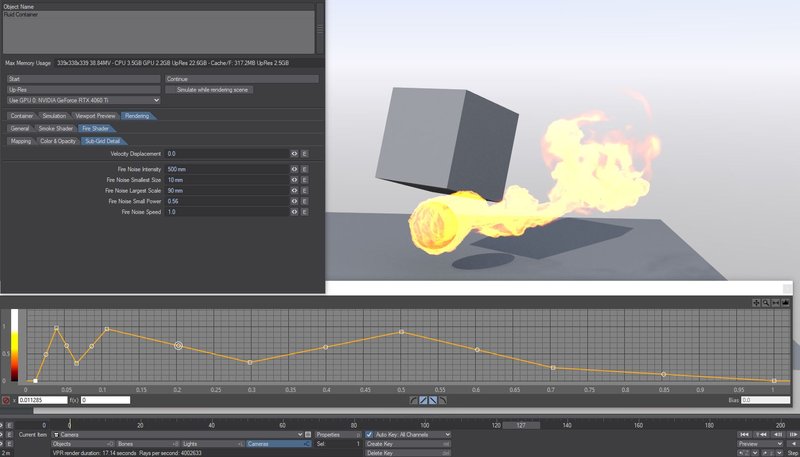
As you can see in the image above with the suggested adjustments to the F-Curve and Sub-grid detail on the Fire Shader, our Fire has more "tooth" and has a better overall color gradient. We can improve the color however by going to the Color & Opacity Sub-Tab and changing some values.
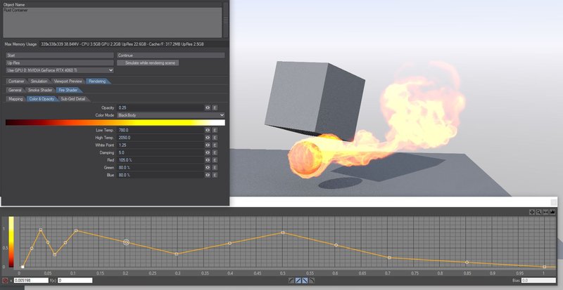
By comparing the two images above and the settings we have now adjusted in the Color and Opacity tab from their default values, we have improved the look of the Fire Shader to be a bit more realistic. Please note the setting change for "Opacity" from the default of 1.0 to 0.25. This helps a lot.
Now let's see what it all looks like together by re-enabling the Smoke Shader.
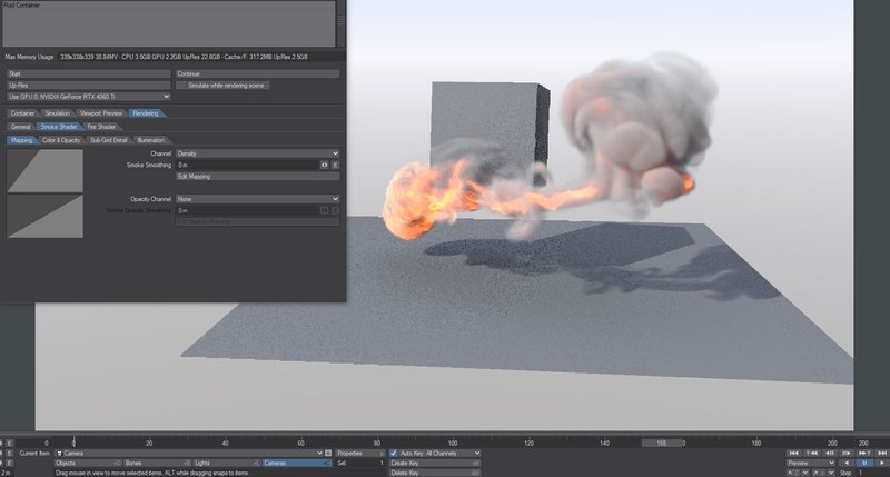
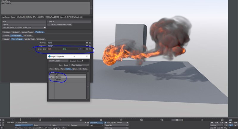
As you can see, scrubbing down the timeline a little bit, that we have our smoke and fire interacting with the Cube (as it is set to be a collision object) and its shaded pretty nicely, but we can improve the look and render speed by doing a couple of things. First off, do we really need to have the smoke illuminated by the default Environment Light? Generally, the answer is no as the multi-scattering function provides a form of "radiosity" from other directional lights in the scene. Second, smoke in nature is made up of carbon particles which are effectively "black" (thus the black body fire shading mode) and we need to reduce the smoke color to a very low setting near "super black" (in video and computer graphics terms) and let just the Distant light do the work for us along with the Fire Shader contributing "light" and thus color to the Smoke Shader. In the image below, we have set the Fluid Container to exclude the Environment Light and we have change the smoke color to RGB = 0.02, 0.02, 0.02. This dramatically improves the look of not only the Smoke but also the Fire.
As demonstrated in this basic workflow guide, it is important to have a fundamental understanding of all of the panels, sub panels and their functions from the emitter creation and settings to simulation and shading step as they work together in a delicate balancing act. It is in many ways a non-linear workflow to achieving a final shot or effect and thus we encourage you to highly familiarize yourself with these areas of TurbulenceFD ahead of time and take a look at our example scenes. Doing so will help you master TurbulenceFD quickly and save you much in the way of time and frustration. We understand that different artists learn different tools in different ways and that is why we have included these example scenes to go along with this documentation so that you can follow along or pull things apart on your own and experiment.