OpenVDB:
New Tools
OpenVDB
Advect Blur
Video about 4 seconds long
Advecting OpenVDB particles with motion blur
New and exciting tools have been added to the LightWave 2020 OpenVDB roster. You now have the ability to bring in Partio particle objects from other software, split and merge your vdb objects for interesting possibilities.
- Advect Points node — Advect particles by velocity grid
- Analysis node — Grid creation Gradient, Curvature, Laplacian, Closest Point, Divergence, Curl, Magnitude, Normalize
- Combine Math node — Combine grids using math operators
- Level Set Morph — Morph between level set grids
- Partio Node — Load Houdini .HClassic particle files
- VectorGrid Split and Merge — Split and merge Vector grids for further experimentation
- Visualize node — Grid viewer with options
The Esc key has been bound to more OpenVDB operations allowing easier cancellation of long operations.
Right now, using Package Scene with a scene with OpenVDB files will package the whole GridCache folder for the content. If you use a single content directory rather than a project-based one you may find that this packaged GridCache folder is enormous and contains far more files than it needs for the one scene. The Package Scene utility will be more intelligent about what it packages in a future release. For now, we thought it was better to package too much rather than not enough when you are transporting scenes.
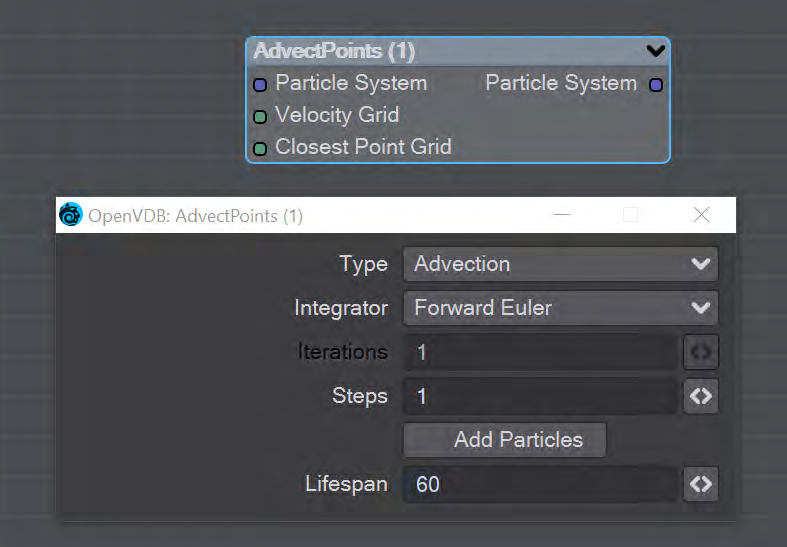
Advect Points node
This node will advect the points in a particle system along a velocity field. The first thing you need is a particle system to use. Node inputs are:
- Particle System - Particle system to advect
- Velocity Grid - This must be a vector-valued VDB primitive. You can use the Vector Merge node to turn a vel. [xyz] triple into a single primitive
- Closest Point Grid - Used for projection and constrained advection
In the node's panel, the controls are as follows:
- Type - Three types are proposed:
- Advection - Move the point along the velocity field
- Projection - Move the point to the nearest surface point
- Constrained Advection - Move the along the velocity field, and then project using the closest point field. This forces the particles to remain on a surface
- Integration - Later options in the list are slower but better at following the velocity field
- Iterations - Number of times to try projecting to the nearest point on the surface. Projecting might not move exactly to the surface on the first try. More iterations are slower but give a more accurate projection
- Steps - How many times to repeat the advection step This will produce a more accurate motion, especially if large time steps or high velocities are present
- Add Particles - At each frame add the input particles to the advection
- Lifespan - How many frames the advected points will live for
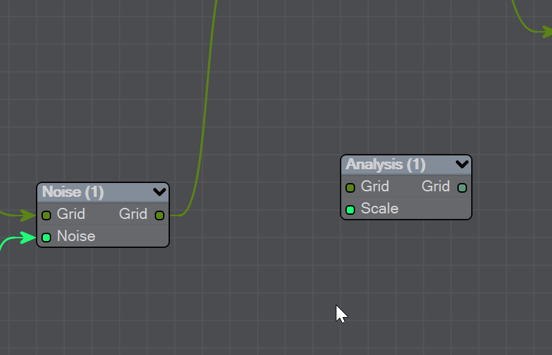
Analysis node
This node presents various grid manipulations. Depending on the input grid type and the operation the output grid type will vary. Once an input is connected and the grid type is known the list of available operations will be collapsed to only show appropriate choices. Finally, if you change the operation the grid output will disconnect (ie scalar to vector).
- Gradient - Vector that points perpendicular to the values basically un-normalized normals (Scalar - Vector)
- Curvature - A measure of the surface curvature (Scalar - Scalar)
- Laplacian - A smoothed version of the input (Scalar - Scalar)
- Closest Point Transform - Direction to the closest point (Scalar - Vector)
- Divergence - A measure of the change in quantities (Vector - Scalar)
- Curl - A direction perpendicular to the input grid vectors (Vector - Vector)
- Magnitude - The scale of the input vectors (Vector - Scalar)
- Normalize - Normalized input vectors (Vector - Vector)
There is also a Scale input for further adjustment.
Combine Math node
Combines grids using scalar operations.
- Combination type - The different math operators that can be brought to bear:
- Copy A - Use A , ignore B
- Copy B - Use B, ignore A
- Invert - Use 1 minus A
- Add - Add the values of A and B (Using Add for fog volumes, which have density values between 0 and 1, will push densities over 1 and cause a bright interface between the input volumes when rendered. To avoid this problem, try using the Blend 2 option)
- Subtract - Subtract the values of B from the values of A
- Multiply - Multiply the values of A and B
- Divide - Divide the values of A by B
- Maximum - Use the maximum of each corresponding value from A and B (Using this for fog volumes, which have density values between 0 and 1, can produce a dark interface between the inputs when rendered, due to the binary nature of choosing a value from either from A or B. To avoid this problem use Blend 1 instead)
- Minimum - Use the minimum of each corresponding value from A and B
- Blend 1 - (1 - A) * B. This is similar to SDF Difference, except for fog volumes, and can also be viewed as a "soft cutout" operation It is typically used to clear out an area around characters in a dust simulation or some other environmental volume
- Blend 2 - A + (1 - A) * B. This is similar to SDF Union, except for fog volumes, and can also be viewed as a "soft union" or "merge" operation. Consider using this over the Maximum or Add operations for fog volumes
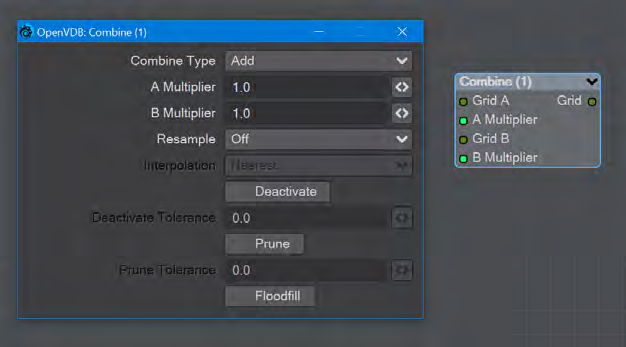
- A Multiplier - Multiply voxel values in the A VDB by a scalar before combining the A VDB with the B VDB
- B Multiplier - Multiply voxel values in the B VDB by a scalar before combining the A VDB with the B VDB
- Resample - Multiple options here. If the A and B VDBs have different transforms, one VDB should be resampled to match the other before the two are combined. Also, level set VDBs should have matching background values (i.e., matching narrow band widths):
- Off - No resampling
- B to Match A - Resample B so that the narrow band width is the same as A
- A to Match B - Resample A so that the narrow band width is the same as B
- Higher-res to Match Lower-res - Resample the higher resolution data so that the resolutions match
- Lower-res to Match Higher-res - Resample the lower resolution data so that the resolutions match
- Interpolation - When you choose a resampling option other than Off, the Interpolation choices become available. There are three to choose between:
- Nearest - Nearest Neighbor interpolation is fast but can introduce noticeable sampling artifacts
- Linear - Linear is the middle ground of speed and quality
- Quadratic - Quadratic interpolation is slow but high-quality
- Deactivate - Toggle to deactivate active output voxels whose values equal the output VDB's background value. When this option is checked, the field below becomes active:
- Deactivate Tolerance - When deactivation of background voxels is enabled, voxel values are considered equal to the background if they differ by less than this tolerance
- Prune - Reduce the memory footprint of output VDBs that have (sufficiently large) regions of voxels with the same value
Pruning affects only the memory usage of a VDB. It does not remove voxels, apart from inactive voxels whose value is equal to the background
- Prune Tolerance - When pruning is enabled, voxel values are considered equal if they differ by less than the specified tolerance
- Flood Fill - Reclassify inactive voxels of level set VDBs as either inside or outside. This option will test inactive voxels to determine if they are inside or outside of an SDF and hence whether they should have negative or positive sign
Level Set Morph
Introduction
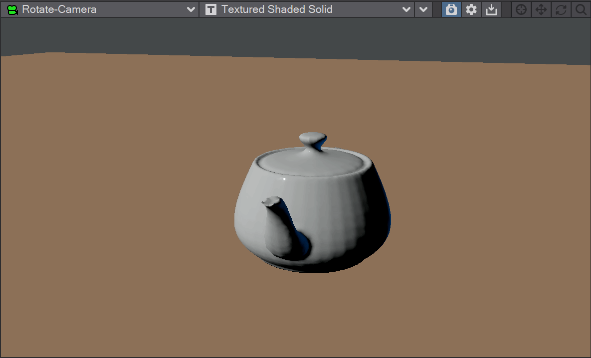
You can morph between polygonal objects. It's not easy because you have to have the same point and poly count, and those points and polygons need to be in the same order; it's a tough job. Now, we have given LightWave the power to do the same using OpenVDB, and as you can see from the rotating teapot/bunny, the results can be very impressive.
You will need to freeze subpatched objects as they are not seen by OpenVDB
Use
In the scene, have two polygonal objects and a null. The point and polygon counts don't have to match, or even be close. In the example above, we are going from the Utah teapot with 1,506 polygons, to the Stanford bunny object with roughly 70,000. Use the Object Replacement > OpenVDB Evaluator entry to convert the two objects to OpenVDB (make sure that their Voxel Size fields match) Level Sets. Pipe the Grid outputs from these nodes into the new Level Set Morph node and from that into the destination Grid node.
Surfaces
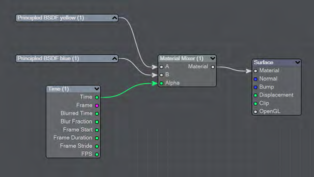
Morphing between objects involves the nodes we've already outlined. Morphing from one surface into another requires the two surfaces be changed as well. To do so, in the Surface Editor, pick your morphing null and edit its surface. Double click on the surface name to open the node editor and add:
- Material Tools > Material Mixer
- The surface for one object
- The surface for the other object
- Info > Time
The node tree will synchronize your surface morphing at the same time as the geometry
Level Set Morph
Level Set Morph
4 second video
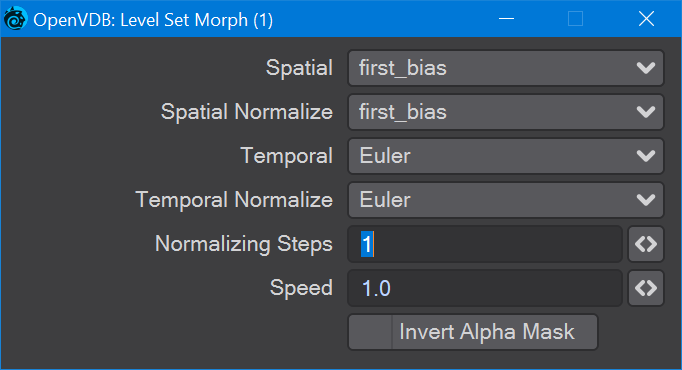
Controls
The first four controls are graded in terms of rapidity and quality. Change up from the first only if it is posing you problems with how the Morph is playing out.
- Normalizing Steps - After morphing the signed distance field, it will often no longer contain valid distances. A number of renormalization passes can be performed to convert it back into a proper signed distance field
- Speed - A scalar to determine how fast your morph occurs
- Invert Alpha Mask - If you have hooked up a grid as an alpha mask, this option allows you to reverse what is alpha'ed out
Partio Node
Introduction
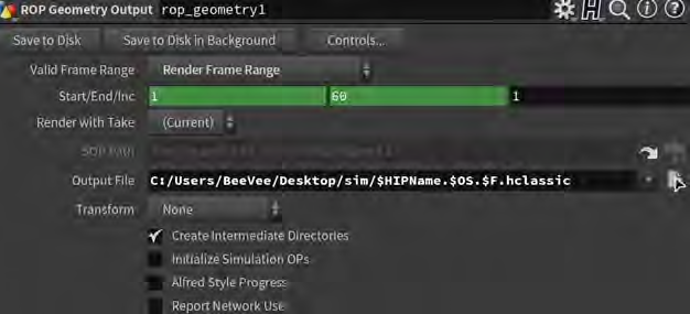
Partio is an open-source C++ library, created by the Walt Disney Animations Studio, for reading, writing and manipulating a variety of standard particle formats (GEO, BGEO, PTC, PDB, PDA). LightWave cannot support the BGEO format, but Houdini can save in the older HClassic format that LightWave will understand. To save in HClassic format, just replace the file extension in Houdini.
Node
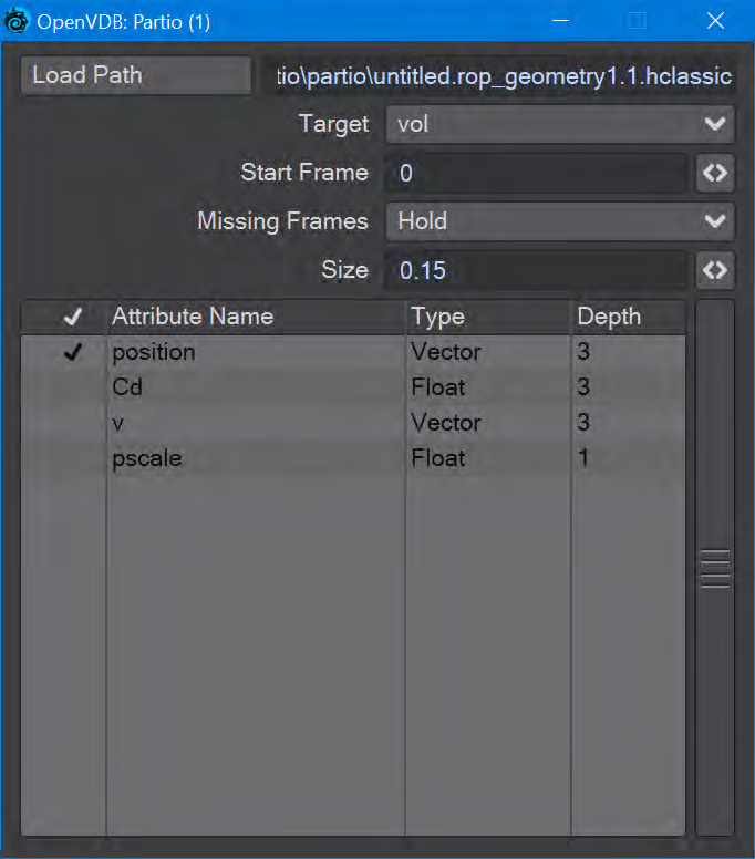
The Partio node is simple in that it has one output and no inputs. Double-clicking on the node shows more depth:
- Load Path - Where your particles are located.
You should place Houdini files in your content directory's GridCache folder to ensure they can be seen by Package Scene.
- Target - If you are using a volumetric object with the particle system, make sure it is targeted here
- Start Frame - The frame on which to start the simulation in LightWave
- Missing Frames - I have Hold (keep the previous frame's contents?) and Blank (leave a gap?)
- Size - The particle size. If using a grid, it should be 1.5 times the voxel size or risk being missed
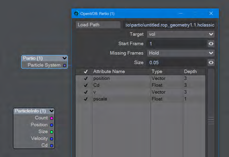
Attributes list
Using the Houdini "vocabulary" here. If you have particles from a different source, the names may be different. The fields are fairly self-explanatory with name, type, and depth. A Float 3 is three scalars, a color for instance. A Float 1 is a simple scalar.
- position - The particle position
- Cd - The diffuse color of the particle
- v - Particle velocity. Can be used as a color or for post blurring, for example
- pscale - The size of the particle
The Partio node has a single output - Particle System. To see these outputs, add an Additional > ParticleInfo node.
Because the outputs are dynamically created, if you are not seeing the outputs you expect, make sure that: • The ParticleInfo node is addressing the right object (double click the node to check the target) • The frame you are on actually has particles. It's not before or after the particles appear • You try stepping the frame forward and back to refresh the node, or moving the ParticleInfo node itself
Usage
Once you have exported a stream of HClassic files, you can import them into LightWave using the Partio node. To do so, add a null to an empty scene. Make the null an OpenVDB Evaluator using the Object Replacement dropdown menu. Hit the P button to edit the Evaluator's nodes. Add the Partio node, but you won't see anything until you have chosen from the following:
There are example Partio scenes in the content in OpenVDB/Partio_Node
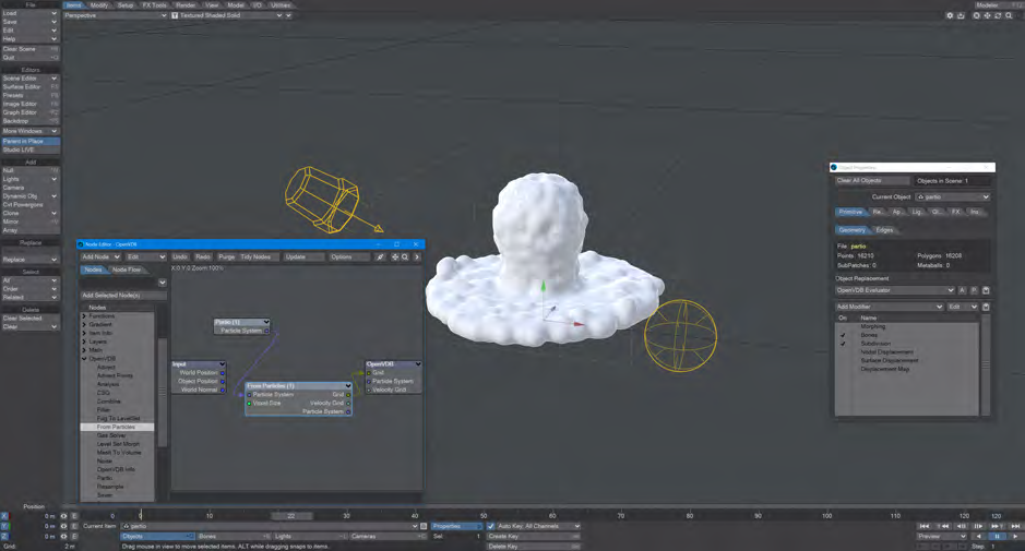
From Particles
Size in the Partio node should be about 1.5 times the Voxel Size in the From Particles node, sometimes a little bigger. This makes sure the particle spans the voxel cube; smaller and you might not see the particle rasterized.
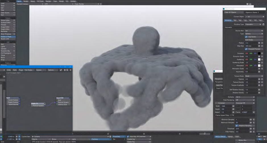
Using the Partio node with a From Particles node
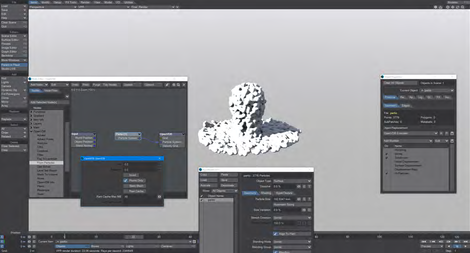
As Particles
You can go straight from the Partio node to the OpenVDB destination node, turn on particles in the destination node and then just get particles that can be used for other purposes - such as with old-fashioned HyperVoxels.
Don't forget to turn on 'Use Legacy Volumetrics' In the Render Properties > Volumetrics tab
LightWave Volumetrics
You can also use LightWave's own Volumetric objects. Add another null called "vol". Set the vol null Primitive Type to Volumetric. Use an OpenVDB Evaluator Object Replacement in the Partio's Object Properties window. In the Node Editor, add a Partio node and bring in your Houdini HClassic files. Set the Partio node Target to the vol null.
Hook the Partio node directly to the Destination OpenVDB node. This will output a particle system. Add a new null labeled "vol" and make it a Volumetric object. Set the source item here to vol.
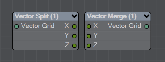
VectorGrid Split and Merge
New to LightWave 2020 is a pair of nodes to split level sets into three separate dimensions for further manipulation. The
Vector Split node takes an incoming OpenVDB grid and splits it into X, Y and Z channels. There is no options panel.
The Vector Merge node will create a vector-valued VDB volume using the values of corresponding voxels from up to three scalar VDBs as the vector components. The scalar VDBs must have the same voxel size and transform; if they do not, use the Resample node to resample two of the VDBs to match the third.
This node offers the following types of operation:
- Tuple - No transformation
- Gradient - Inverse-transpose transformation, ignoring translation
- Unit Normal - Inverse-transpose transformation, ignoring translation but with renormalization
- Displacement - Transformation, ignoring translation
- Position - Transformation with translation
- Copy Inactive Values - If enabled, merge the values of both active and inactive voxels. If disabled, merge the values of active voxels only, treating inactive voxels as active background voxels wherever corresponding input voxels have different active states
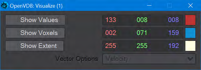
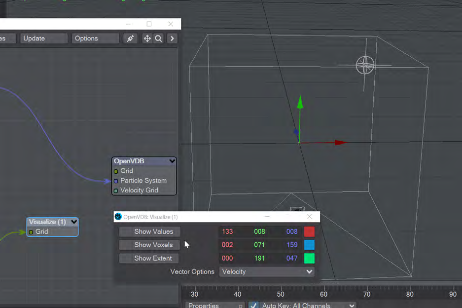
Visualize node
Additional Destination node to help visualize VDB networks. You can choose any combination of the three choices -Values, Voxels, and Extent. When this node uses a Velocity Grid output as its input, the Vector Options dropdown menu becomes available.
- Show Values - Shows the scalar voxel values multiplied by color
- Show Voxels - Show the voxel cubes
- Show Extent - Puts a box surrounding the voxel object showing the extents
- Vector Options - A dropdown menu with three options. This menu is ghosted when the Visualize node is not hooked to a Velocity Grid
- Velocity - Shows velocity unclamped transformed
- Normal - Shows normals scaled to .4 of box size to prevent overlap. Inverse transformed
- Color - Shows the color with no transform